Allowing Remote Connections to SQL Express (the Right Way) (Video)

Sometimes we need to allow remote connections to a SQL Server Express or Developer edition instance, usually on our local machine. In this video demo, I show you how to allow remote access without resorting to disabling the Windows Firewall entirely, which is an unfortunately-common solution pervading the internet.

Since there are many possible configurations (which is why I say “default” a lot in the video — sorry), and part of what I covered applies to all editions of SQL Server, a much more complete reference can be found here on MSDN.

Efficiently Indexing Long Character Strings

Sometimes we face the requirement to search a table for a specific string value in a column, where the values are very long. The default answer is to create an index, but we must remember that index keys cannot exceed a 900-byte size limit, and LOB columns (which include the MAX type variants) cannot be in the index key at all. In this post, we’ll explore a method to efficiently index long character strings where the search operation is moderately-to-highly selective.

The Methodology

Since we’re faced with a size restriction on the index key (or the string column cannot be included in the key at all), we need to apply some kind of transformation to the string data to make its representation — and hence the index key size required — smaller.

Of course, we can’t simply compress an infinite amount of data into a comparatively very small field, so the index we create won’t be able to support all the same operations as if we had indexed the original field. But most of the time, that isn’t a problem — generally, we need to search for an exact match, or a string starting (or maybe even ending) with a given few characters.

We’re going to do this by performing a computation on the original values, storing the result in a new column in the table, and creating an index on that column (there are two ways to do this, which we’ll get into shortly). In terms of the computation itself, there are a few different options that can be used, depending on what needs to be accomplished. I’ll introduce two basic approaches here, and then we’ll run through some code that demonstrates one of them.

  1. Use the LEFT function to grab the first several characters and discard the rest. This method is appropriate for both exact matching and wildcard searching with a few given characters (i.e., LIKE ‘abc%’), and because the original text stays in tact, it supports case/accent-insensitive matching without doing anything special. The drawback of this method, though, is that it’s really important to know the data. Why? To improve the efficiency of queries, the number of characters to use should be enough such that the computed values are more or less unique (we’ll see why in the example). It may in fact be the case that the original field always has a consistent set of characters at the beginning of the string (maybe they’re RTF documents or something), so most of the computed values would end up being duplicates (if that’s the case, this approach won’t work and you’ll want to use the other approach instead).
  2. Use a traditional hash function (such as HASHBYTES) to compute a numeric representation of the original field. This method supports exact matching (case-insensitivity with a small tweak, and accent-insensitivity with a bit of code), but not partial matching because the original text is lost, and there’s no correlation between the hash value and the original text. It’s also critical to watch the data types involved here, because hash functions operate on bytes, not characters. This means hashing an nvarchar(MAX) value N’abc’ will not give the same result as hashing a varchar value ‘abc’, because the former is always 2 bytes per character. Those are the downsides. The upside is that traditional hashing has the ability to work on data that contains very few differences, and when the text starts with the same sequence of characters.

Both of these methods are hash functions, as they convert a variable length input to a fixed length output. I suppose the first approach isn’t technically a hash function because the input could be shorter than the number of characters desired in the output, but I think you see my point that both approaches “sample” the original data in a way that allows us to represent the original value more or less uniquely without needing to carry around the original data itself. Maybe it’s more correct to speak of them as lossy compression algorithms. In any event, I will refer to the results of these functions as hash values for the remainder of the post.

Because this method omits some (or probably most) of the original data, some extra complexity in our code must be introduced to compensate for the possibility of duplicate hash values (called a hash collision). This is more likely to happen using the first approach as the original data values are partially exposed. It’s still possible, however rare, that the second approach can have duplicates, too, even if the input text is unique, so we must accommodate for that.

Speaking specifically about using a traditional hash function, such as HASHBYTES, there are a couple major things to consider. First, there are several different algorithms to choose from. Because we aren’t going to be using the hash value for any type of cryptographic functionality (i.e., we don’t care about how difficult it will be to “unhash” the values), it’s largely irrelevant which algorithm we choose, except to pick one that produces a hash value of an acceptable size. A larger hash value size will reduce the possibility of collisions as there are more possible combinations, but as I already mentioned, we have to handle for collisions anyway because no hash function is perfect; therefore, it’s okay to use a smaller hash value size to save storage space, and pick a hash algorithm that is least expensive to compute initially.1

Second, we need to make sure that the hash values represent a consistent portion of the string input values. HASHBYTES is great because it’s built-in, but its input parameter is limited to 8000 bytes. This means if the string values needed to be hashed are longer than 8000 char/4000 nchar, a slightly different approach should be taken. I would recommend creating a CLR scalar function, as there are no limitations of input size in the .NET hashing classes.

The Test

As I mentioned previously, there are two ways to store the hash values so they can be indexed:

  1. Computed column. This method has two advantages: first, the SQL Server engine automatically keeps the hash value up-to-date if the source column changes. Second, if we use a non-PERSISTED column, we save the storage space for the hash values in the base table. The main disadvantage is that we may have to poke and prod our SQL statements to get the plan shape we want; this is a limitation of computed columns in general, not of what we’re doing here specifically. Note: if your goal is to create hash values in two tables and JOIN them together on that column, it may not be possible to do it efficiently using computed columns because of bizarre optimizer behaviour. Any time computed columns are involved, always inspect the execution plan to make sure SQL Server is doing what’s expected — sometimes common sense doesn’t make it into the execution plan that gets run.
  2. Base table column, updated by triggers (if required). This method works best to get execution plan shapes that we want, at the expense of a bit of complexity to keep the values updated, and the additional storage space required in the base table.

In the example below, we’ll use the base table column method, as it’s the most flexible, and I won’t have to go into detail about hinting in the SQL statements.

Let’s start by creating a table to play with:

CREATE TABLE [dbo].[Table1]
(
	Id int NOT NULL IDENTITY
		PRIMARY KEY CLUSTERED,
		
	StringCol varchar(MAX) NOT NULL
);
GO

And then we’ll populate it with some test data (note: the total size of the table in this demo will be about 70 MB):

SET NOCOUNT ON;
GO

INSERT INTO [dbo].[Table1](StringCol)
	SELECT
		REPLICATE('The quick brown fox jumps over the lazy dog. ', 5) +
			CONVERT(varchar(MAX), NEWID())
		FROM master..spt_values v
		WHERE v.type = 'P';
GO 64
	
INSERT INTO [dbo].[Table1](StringCol)
	VALUES ('The quick brown fox jumps over the lazy dog.');
GO 3

So we’ve got about 130,000 random-type strings, and then 3 rows which we can predict. Our goal is to efficiently find those 3 rows in the test queries.

Since the string field was defined as varchar(MAX), we can’t create an index on that column at all, and the only index we have in the base table is the clustered index on the Id column. If we try a naive search at this point, we get a table scan, which is the worst case scenario:

DECLARE @search varchar(MAX) =
	'The quick brown fox jumps over the lazy dog.';

SELECT Id, StringCol
	FROM [dbo].[Table1]
	WHERE StringCol = @search;

Indexing Long Character Strings 1

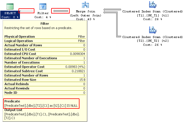
We get our 3 rows back, but this is far from ideal. I’m not sure why the optimizer chooses a scan and filter instead of pushing down the predicate into the scan operator itself, but that’s beside the point because this is an awful plan, with an estimated cost of over 3.5.

Let’s move on and create our hash value column and populate it. Note that if you want to update the hash values using triggers and keep the column NOT NULL, you’ll need to add a default constraint so INSERTs don’t fail outright before the trigger code gets a chance to run.

ALTER TABLE [dbo].[Table1]
	ADD StringHash binary(16) NULL;
GO
	
UPDATE [dbo].[Table1]
	SET StringHash = CONVERT(binary(16), HASHBYTES('MD5', StringCol));
GO

ALTER TABLE [dbo].[Table1]
	ALTER COLUMN StringHash binary(16) NOT NULL;
GO

We have our hash values in the table, but still no index to improve our query. Let’s create the index now:

CREATE NONCLUSTERED INDEX IX_Table1_StringHash
	ON [dbo].[Table1](StringHash);

While this looks unremarkable, the index has been created non-unique on purpose — first and foremost to accommodate duplicate source (and hence hash) values, but also to allow for the possibility of hash collisions. Even if your source values are guaranteed unique, this index should be non-unique. Other than that, this should be enough to let us construct a query to make the search more efficient:

DECLARE @search varchar(MAX) =
	'The quick brown fox jumps over the lazy dog.';

SELECT Id, StringCol
	FROM [dbo].[Table1]
	WHERE
		(StringHash = CONVERT(binary(16), HASHBYTES('MD5', @search))) AND
		(StringCol = @search);

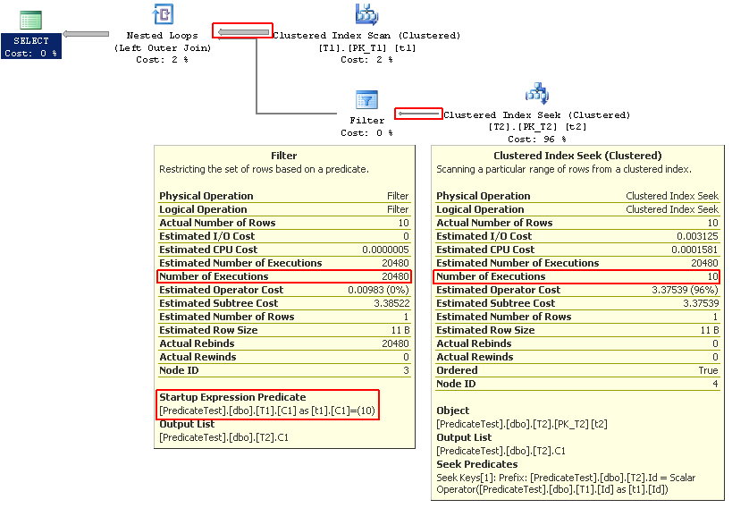
You’ll notice I’ve still included the StringCol = @search predicate in the WHERE clause — this is to ensure correct results of the query due to hash collisions. If all we did was compare the hash values, we could end up with extra rows in the results. Here’s the execution plan of the query above:

Indexing Long Character Strings 2

We got an index seek, which was the main thing we were looking for. The Key Lookup is expected here, because we have to compare the original values as well, and those can only come from the base table. You can now see why I said this method only works for moderately-to-highly selective queries, because the key lookup is required, and if too many rows are being selected, these random operations can kill performance (or the optimizer may revert to a table scan). In any event, we now have an optimal query, and even with the key lookups happening, the estimated cost was 0.0066, an improvement by over 500x on this smallish table.

Takeaways

I’m sure at this point you can think of several other uses for this methodology; it can be applied to large binary fields, too. You could even implement it for cases where the column could be indexed directly (say, varchar(500), with most of the values taking up nearly all the allowed space), but maybe you don’t want to — hashing the data might save a significant amount of storage space, of course at the expense of code complexity and a bit of query execution time.

While hashing data is nothing new, this technique exploits hashing to greatly improve the efficiency of data comparisons. I’ll leave it as an exercise for the reader to try the JOINing scenario I mentioned above — if you do, try it using computed columns first for maximum learning — you’ll find that this technique also improves the queries, as long as the join cardinality remains low (like in the 1-table scenario, to control the number of key lookups).


1 While I haven’t tested this in SQL Server either using HASHBYTES or a CLR function, there are implementations of certain hash algorithms in processor hardware itself. This may be of benefit to reduce CPU usage, possibly at the expense of storage depending on the algorithms in question.

Row Filter Operators vs. Startup Expression Operators

In a previous post, I introduced how to use startup expression predicates in T-SQL queries to improve performance. Based on the feedback I got, there was some confusion about what this operator actually does, and why it appears in the query plan as a Filter operator, which is usually seen in other contexts. In this post, I’ll explain the differences and similarities of the Row Filter operator (which is seen more typically) and the Startup Expression filter operator.

Comparison By Example

Let’s set up a test scenario that can be used to demonstrate and compare the two types of operators (note: the test data is <1 MB):

SET NOCOUNT ON;

CREATE TABLE [dbo].[T1]
(
	Id int IDENTITY
		CONSTRAINT PK_T1 PRIMARY KEY,
	C1 int NOT NULL
);

CREATE TABLE [dbo].[T2]
(
	Id int IDENTITY
		CONSTRAINT PK_T2 PRIMARY KEY,
	C1 int NOT NULL
);
GO

INSERT INTO [dbo].[T1](C1)
	SELECT number FROM master..spt_values WHERE type = 'P'; /* 0-2047 */

INSERT INTO [dbo].[T2](C1)
	SELECT number FROM master..spt_values WHERE type = 'P';

GO 10

Now we can try running a couple queries to see these operators in action. Here’s the first one, which contains a Row Filter predicate (like the previous post, I’m using hints so you can reproduce the same plans more easily if you try this yourself):

SELECT
	t1.C1,
	t2.C1
	FROM [dbo].[T1] t1
	LEFT OUTER MERGE JOIN [dbo].[T2] t2 ON t2.Id = t1.Id
	WHERE t2.C1 IS NULL
	OPTION(FORCE ORDER);

And here’s the execution plan (click for full size):

Row Filter vs Startup Expression 1

As we can see, the query joined the two tables together, and then filtered that set of rows to give the final result.

The Row Filter operator evaluated the predicate against each returned row (the big arrow to the right of the operator), and output only the rows where the predicate evaluated to true (no rows in this case; the small arrow to the left of the operator).

Here’s the next query, which uses a Startup Expression predicate (this query isn’t logically equivalent to the first one):

SELECT
	t1.C1,
	t2.C1
	FROM [dbo].[T1] t1
	LEFT OUTER LOOP JOIN [dbo].[T2] t2 WITH(FORCESEEK) ON
		(t1.C1 = 10) AND
		(t2.Id = t1.Id)
	OPTION(FORCE ORDER);

And here’s the query plan:

Row Filter vs Startup Expression 2

This time, table T1 was scanned (20480 rows), and the Startup Expression filter operator was executed for each of those rows. However, the index seek to table T2 was only executed 10 times. How did that happen?

The Startup Expression filter evaluated the predicate against each request row coming in from the upper input (in this case the T1 table scan), and only propagated the request where the predicate evaluated to true. This is how a Startup Expression operator “protects” or  “guards” operators to its right, so they aren’t executed for every request row. While this particular example is contrived, it’s this “guarding” that improves performance by only executing the subsequent operator branch the minimum number of times necessary.

Summary

Both the Row Filter operator and Startup Expression filter operator evaluate a predicate against rows.

The Row Filter operator applies the predicate to returned rows, returning only the rows that match the predicate, while the Startup Expression filter operator applies the predicate to requested rows, only making further requests when the row matches the predicate.

While both operators perform essentially the same work (hence they both appear as a Filter operator), they do so logically reversed of each other, and therefore perform very different functions within a query plan.

Is my SQL Server’s memory over-committed?

As our applications’ data grows, so usually does the memory required by SQL Server to efficiently process requests for that data. Sometimes those requirements are more than the host operating system instance can handle, and we don’t find out about it until it’s too late and performance takes a nosedive. In this post, we’ll explore what memory over-commit is and why it’s a bad thing, how to mitigate the problem, and how to help prevent it from occurring in the first place.

Cause

It’s pretty obvious that memory over-commit occurs when the amount of memory required by applications exceeds the amount of physical memory available in the host operating system. (This applies equally to both physical and virtual machines. In this post, when I say “host operating system,” I mean an operating system instance that hosts SQL Server, not an operating system instance that hosts virtual machines.)

When the amount of memory required exceeds the amount of physical memory available, Windows uses disk (the page file) as a persistent store to satisfy the excess memory requirements. This is why this mechanism is called Virtual Memory — it looks like normal memory to an application, but really Windows is backing it with disk.

How does this happen? Well, first, you’ll notice that I haven’t mentioned anything directly about SQL Server. Virtual Memory is a mechanism of Windows, and so it applies to all applications that run under Windows, including SQL Server. In fact, it’s possible the system is over-committed because of memory requirements from applications other than SQL Server. Usually, though, SQL Server is the largest consumer of memory in a Windows instance, so it’s also usually responsible for causing over-commit problems.

The heart of the issue is controlling the amount of memory SQL Server is allowed to allocate. The only real influence we have over this is the Max Server Memory setting. While that might sound really concrete, the problem is that it… doesn’t actually control the total amount of memory SQL Server can allocate. On SQL Server 2005 to 2008 R2, this setting controls the maximum amount of memory used for the buffer pool only; it doesn’t include other memory pools such as the procedure cache, which can be very significant (gigabytes!) in some scenarios. SQL Server 2012 improves the state of affairs by increasing the scope of what this setting covers. While it’s still not perfect, it’s a welcome improvement to better represent what the setting actually does, and offers greater control of maximum memory utilization. In any event, the point is that this setting underestimates the amount of memory that’s going to be used (sometimes significantly, as mentioned), which can lead to unexpected over-commit.

Symptoms

The performance implications of backing memory with disk can be crippling: disk can be thousands of times slower than physical memory, particularly when it comes to where the Windows page file is landed, as we don’t normally put it on our fastest, most expensive storage device. Probably the worst-case scenario is when the page file is landed on a RAID 1 mirror (the typical physical machine scenario), which simply isn’t meant to handle a huge number of random reads or writes.

In order to detect when memory over-commit is happening, you’ll have to be doing Performance Monitor (PerfMon) logging, as you really won’t see anything directly in SQL Server except that things are very slow (more accurately, the wait time associated with retrieving a page from the buffer pool without physical I/O will be high). I strongly recommend setting up 24/7 PerfMon logging in your environment, and at some point I’ll write a post or record a demo video of how to set it up.

Below are the key PerfMon counters you’ll want to record to detect and troubleshoot memory over-commit. This, of course, is by no means an exhaustive list of all the counters you should be recording.

  • Paging File(_Total)\% Usage – Not surprisingly, this counter can be a dead giveaway to detect if there are issues. If it’s at any value greater than zero, you need to take a closer look at the other counters to determine if there’s a problem. Sometimes a system will be perfectly fine with a value less than 2-3% (it also depends on the size of the page file), but the higher this counter is, the more of a red flag it is. Also, watch this counter to make sure it’s stable, and not creeping up over time.
  • Memory\Available MBytes – If this number is below ~500 (in the absence of page file usage), you’re in the danger zone of over-commit. It’s recommended to keep at least this much memory available not only for unexpected SQL Server usage, but also to cover the case where administrators need to Remote Desktop into the box for some reason. User sessions take memory, so we need to keep some free for emergencies. I won’t get into the amount of memory to keep free on a SQL Server here, as that’s a discussion in itself. My point here is that if this counter is getting too low (less than ~500), you could start getting in trouble soon. I should note also that if the system is currently over-committed, this counter will reflect the amount of virtual memory provisioned, as it gets counted as available memory. So the system could be over-committed, yet appear to have plenty of available memory — look at the other counters to put the number in context.
  • Physical Disk\Disk Reads/sec and Physical Disk\Disk Writes/sec for the disk that has the page file on it – Normal operations do cause some disk activity here, but when memory over-commit happens, these counters will spike up dramatically from the baseline.

Since memory over-commit can only happen when the amount of physical memory is exhausted, the system will only become slow after a certain point. In troubleshooting, sometimes a SQL instance (or Windows itself) is restarted, and it fixes the problem for a while, only to return some time later. By now it should be obvious that this happens because after a restart, the SQL Server buffer pool is empty, and there’s no possibility of over-commit until the physical memory is used up again.

Solution

Iteratively lower SQL Server’s Max Server Memory setting (or initially set it to a reasonable value), and monitor the performance counters until the system falls back to a stable configuration. Because of the nature of Virtual Memory, Windows can hold on to swapped-out pages for quite a long time, so it’s possible that the counters will stabilize with the page file usage at a higher level than normal. That may be okay, as when the pages are swapped back in, they will never be swapped out again, unless the settings on this iteration are still out of whack. If the initial configure was way off (default Max Server Memory setting), you may want to restart the box to start with a clean slate, because the counters will be so far out.

It seems counter-intuitive to lower the amount of memory SQL Server is able to allocate. SQL Server internally manages which sets of pages in memory are hot and cold, an insight Windows doesn’t have. This means that by adjusting the Max Server Memory setting down, even though the amount of memory available to SQL Server will be less, it will still be able to perform well by keeping the most active pages in memory, and only going to physical disk occasionally for pages that aren’t in the buffer pool, as opposed to potentially going to disk for any memory access.

Prevention

While over-commit can never truly be prevented — users could potentially run other applications on the SQL box that require lots of memory — what you can put in place is an early-warning system by monitoring the PerfMon counters. Third-party software solutions should be able to help with this, particularly if you manage many servers.

Speaking of other applications, if you have any installed on the SQL box (including the third-party monitoring software I just mentioned), it’s doubly important to monitor the state of affairs, as these are variables out of your control. The Max Server Memory setting and the amount of available member should be more conservative in this case.

It’s also important, particularly if your SQL Server is version 2005 to 2008 R2, to ensure the Max Server Memory setting is allowing for some future growth in your environment. Because the setting doesn’t encompass the plan cache, even adding an insignificantly-small database could cause over-commit if many different queries are run against it. The setting and counters should be evaluated as part of the change process. For SQL Server 2012, this is less of a concern for the reasons previously mentioned, but it can still be worth checking things out as part of your regular change process.

Finally, try to avoid letting users remote into the SQL box to do regular work or maintenance, as this can use up a tremendous amount of memory. Nearly all tasks can be accomplished remotely using SQL Server Management Studio and remotely/non-interactively using PowerShell. If your administrators’ workstations aren’t in the same domain as your servers, create a management box on the server domain, and remote into that instead to manage the servers.

Startup Expression Predicates

When we write T-SQL statements, what we’re really doing is describing what data to return. It’s then up to the internals of SQL Server to best decide how to most efficiently return the data we asked for.

Sometimes, there’s extra information we know about, but that SQL Server doesn’t (automatically). Letting SQL Server in on this seemingly redundant information can change how efficiently the data is accessed and returned.

In this post, we’ll walk through a simple parent/child example that exploits a partially denormalized table schema to improve join performance to the child tables. The performance improvement comes through SQL Server producing query plans that contain Startup Expression Predicates, which effectively prevents certain parts of the query plan from executing in some cases.

Test Setup

The first thing we need to do is set up the tables. We’ll need a ProductTypes table, a parent table (Products) and two child tables (ItemProducts and ServiceProducts).

CREATE TABLE [dbo].[ProductTypes]
(
	Id tinyint NOT NULL PRIMARY KEY,
	Description varchar(50) NOT NULL
);

CREATE TABLE [dbo].[Products]
(
	Id int NOT NULL PRIMARY KEY,
	ProductTypeId tinyint NOT NULL
		FOREIGN KEY REFERENCES [dbo].[ProductTypes](Id),
);

CREATE TABLE [dbo].[ItemProducts]
(
	ProductId int NOT NULL PRIMARY KEY
		FOREIGN KEY REFERENCES [dbo].[Products](Id),

	ItemColumn int NOT NULL
);

CREATE TABLE [dbo].[ServiceProducts]
(
	ProductId int NOT NULL PRIMARY KEY
		FOREIGN KEY REFERENCES [dbo].[Products](Id),

	ServiceColumn int NOT NULL
);

In this type of design, there will only ever be a single row in one of the child tables for each row in the parent table. This is typically handled by some form of business logic (stored procedures or views) and enforced by constraints, but I want to keep this example simple, so I’m only mentioning this for the sake of completeness, and what the data is going to “look” like.

Okay, let’s add some test data so we can run some queries:

INSERT INTO [dbo].[ProductTypes](Id, Description)
	VALUES
		(1, 'Item'),
		(2, 'Service');
		
INSERT INTO [dbo].[Products](Id, ProductTypeId)
	VALUES
		(1, 1),
		(2, 2);
		
INSERT INTO [dbo].[ItemProducts](ProductId, ItemColumn)
	VALUES (1, 50);
	
INSERT INTO [dbo].[ServiceProducts](ProductId, ServiceColumn)
	VALUES (2, 40);

Now we have rows representing one ItemProduct, and one ServiceProduct.

Querying the Data

First let’s start by looking at a typical query that might be run against these tables:

SELECT
	p.Id AS ProductId,
	p.ProductTypeId,
	COALESCE(ip.ItemColumn, sp.ServiceColumn) AS OtherColumn
	FROM [dbo].[Products] p
	LEFT OUTER JOIN [dbo].[ItemProducts] ip WITH(FORCESEEK) ON
		ip.ProductId = p.Id
	LEFT OUTER JOIN [dbo].[ServiceProducts] sp WITH(FORCESEEK) ON
		sp.ProductId = p.Id;

(Note: the hints are not standard, but are needed for demonstration purposes; I got a nested loops/table scan plan by default. See the final section of this post for some extra discussion.)

Since each product row will only exist in one of the child tables, we have to use LEFT joins to get any results. The query plan looks like this (click for full size):

Startup Expression Predicates 1

We can see that for each row in the Products table, SQL Server must join to both child tables in case there are rows there. Legitimately there could be, as the only thing preventing that is our business logic. SQL Server doesn’t understand that, so it has no choice but to ensure correctness and do the extra work.

Here’s where the magic comes in. We know that for a given ProductTypeId, rows will only exist in one of the child tables. If SQL Server knew that, then it would only have to join to one child table for each row in Products.

Let’s try this query:

SELECT
	p.Id AS ProductId,
	p.ProductTypeId,
	COALESCE(ip.ItemColumn, sp.ServiceColumn) AS OtherColumn
	FROM [dbo].[Products] p
	LEFT OUTER JOIN [dbo].[ItemProducts] ip WITH(FORCESEEK) ON
		(ip.ProductId = p.Id) AND
		(p.ProductTypeId = 1) /*****/
	LEFT OUTER JOIN [dbo].[ServiceProducts] sp WITH(FORCESEEK) ON
		(sp.ProductId = p.Id) AND
		(p.ProductTypeId = 2) /*****/

Now we’re telling SQL Server something about our business logic. Let’s see if this improves the execution plan:

Startup Expression Predicates 2

That’s better. SQL Server has added two Filter operators — one for each child table — that reject rows that don’t satisfy the Startup Expression Predicate (in other words, the extra business logic we told SQL Server). This results in only a single seek against the proper child table for each row in the Products table. This could provide a big performance boost: for the number of child tables (m) and the number of parent rows (n), this approach will always execute only n seeks (thus making the number of seeks independent of the number of child tables), instead of m*n as the first approach does. This does of course come at the penalty of storage to denormalize enough information (ProductTypeId in this case) to drive the process, but usually that’s not going to be a huge hit (most likely 1 byte per row in the parent table).

As a bonus, here’s a different approach to writing the same query. This form may be more appropriate for some things, depending on what you’re trying to do:

SELECT
	p.Id AS ProductId,
	p.ProductTypeId,
	a.OtherColumn
	FROM [dbo].[Products] p
	CROSS APPLY
	(
		SELECT
			ItemColumn AS OtherColumn
			FROM [dbo].[ItemProducts] ip
			WHERE
				(ip.ProductId = p.Id) AND
				(p.ProductTypeId = 1) /*****/
				
		UNION ALL
		
		SELECT
			ServiceColumn
			FROM [dbo].[ServiceProducts] sp
			WHERE
				(sp.ProductId = p.Id) AND
				(p.ProductTypeId = 2) /*****/
	) a;

And here is the resulting query plan that contains the Startup Expression Predicate Filter operators:

Startup Expression Predicates 3

Conclusion

Sometimes giving SQL Server more information than you might think is necessary can help to improve the query plans that are generated. Certainly in cases like this parent/child example, we were able to exploit a denormalized ProductTypeId column to drive the index seeks to the child tables, and make the query scale much better. The result in this case was that the total number of seeks against the child tables became independent of the number of child tables, while still retaining the original query logic. Look for opportunities like this in your queries to give SQL Server extra hints about your table schema — you can be rewarded with more scalable queries.


More?

As I was playing around with these examples, in particular the second query, I found it interesting that for some reason if the plan used a scan operator as the lower input of the nested loops join (such as I got by not using the FORCESEEK hints), there were no startup expression predicates to be found (nor Filter operators). Instead, the predicate end up on the nested loops operator itself, with each child table scanned for every upper input row. This is somewhat puzzling, as I can’t think of a reason why the lower input couldn’t be protected by a startup expression in that scenario as well. (Note: I only tested on a 2008 R2 RTM instance.)